Filling in the holes: Generating point estimates for QCEW suppressed data

Economic Research Analyst, Indiana Business Research Center, Indiana University Kelley School of Business

Data suppression for industries at the county level creates a challenge that researchers are using data science techniques to overcome.

Overview

Regional economic researchers use public data extensively in their work—for example, to study sectoral employment growth across U.S. regions. While data on companies (aka establishments) at the national, state and metropolitan area levels are largely accessible, data for more granular geographies, such as county or city, are often suppressed in order to protect against identifying specific establishments. Data suppression is more likely in less populous areas or when seeking very specific industries, such as higher-digit North American Industry Classification System (NAICS) codes.¹ This leads to research with either limited geographic scope or less-specific industrial classifications—or both. Consequently, the lack of granular data limits the utility of the research for practitioners.

Two public sources for county-level industrial data are used most frequently by researchers: County Business Patterns (CBP), an annual product of the U.S. Census Bureau, and Quarterly Census of Employment and Wages (QCEW), a quarterly and annual product of the U.S. Bureau of Labor Statistics (BLS).

In describing the various employment data sets, the U.S. Bureau of Economic Analysis website explains that the CBP data on employment and payrolls are annual extensions of the Census Bureau’s five-year economic censuses and are derived from federal administrative records and survey information from business establishments that comprise the Census Bureau’s business registry. The BLS data on county employment and wages are derived from the monthly/quarterly administrative records of state unemployment insurance (UI) legislation and, for the case of federal employees, of the federal unemployment compensation program (UCFE).²

Although CBP provides data at more granular levels, such as ZIP codes, we favor QCEW because it is more up to date, more comprehensive—pulling data from a larger number of establishments—and thus potentially more accurate.³

That said, data suppression in QCEW is significant. Manufacturing data for 2016 is an example. Across all U.S. counties, only 12 percent of the QCEW manufacturing employment data are suppressed at the two-digit NAICS level. However, that number increases sharply to 57 percent for the three-digit codes, and continuously climbs up to 89 percent for the six-digit codes (see Figure 1). Thus, “filling these holes” becomes a necessary, yet challenging, task.

Figure 1: Percent of manufacturing employment that is suppressed at the U.S. county level, 2016

Source: U.S. Bureau of Labor Statistics, using QCEW data

For reference, here is a screenshot of what just a couple of industries look like as coded by NAICS—starting at the four-digit level:

View the complete 2017 NAICS »

Researchers have been increasingly using data science techniques to estimate the suppression in these cells. The Indiana Business Research Center (IBRC) is among those estimating those suppressed data since a significant portion of our research relies on both county-level data and detailed industrial data.

A summary of the IBRC method

We handle the suppressed cells in two phases:

• Phase 1—The Range Finder: We calculate the range (the minimum and maximum values) for each suppressed cell based on its bounded margins at the county, state, national and industry level. We generate these across 10 cycles or iterations using machine-learning techniques. These iterations⁴ are necessary since the ranges for all other suppressed cells are then adjusted every time a new range is revealed.
• Phase 2—The Point Finder: Here, we calculate the actual point estimates for suppressed cells using the input-output table compilation method (aka RAS algorithm), incorporating the results of the Range Finder. To ensure accuracy, our estimation process takes a top-down approach—starting from the two-digit and working down to the six-digit NAICS codes.⁵ More detail on the RAS algorithm is available at the end of this article.

We also integrate data from other trustworthy public sources (for example, cells suppressed in QCEW are not always suppressed in the CBP data). We run the model separately for each year of data back to 2001 (when the QCEW data were first released using NAICS codes).

The result is what we call the QCEW-Complete time series, which is also smoothed (so as to tamp down any large spikes or dips).

A look at the results

We conducted a validity check of our estimates with the Indiana “truth,” pulled from state administrative records. We were able to confirm that the estimates were improved through increasingly granular levels of detail (from two-digit through six-digit).

At the two-digit NAICS level, 24 percent of the industries we estimated deviated from their true employment by more than 50 percent (either 50 percent above or 50 percent below true value). These numbers increase to around 55 percent for higher-digit NAICS codes. Since these industries tend to be small establishments with fewer than 10 employees (for the five- and six-digit NAICS level), scale wise, these deviations are not substantial.

The primary reason for data suppression in public data is to protect identities and to prevent wrongful use of such data. This, on the other hand, jeopardizes the good use of such data—by researchers and local developers—due to a large amount of missing information.

The IBRC has been using the QCEW-Complete data set to conduct research and provide regional and local economic developers and workforce professionals with tools to discover their economic opportunities and challenges. A good example is the Regional Labor Mix on Hoosiers by the Numbers, a data tool created and maintained by the IBRC in collaboration with the Indiana Department of Workforce Development. Overall, policy initiatives backed by research done with the QCEW-Complete data can help ensure a better understanding of local economies and prevent faulty decision making.

More on the method: The RAS algorithm

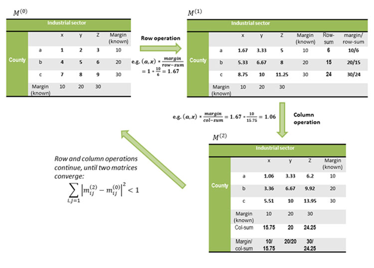
The RAS algorithm⁶ is one type of “iterative proportional fitting” procedures. Here’s the basic idea: In a situation where the sums of data entries (on an input table) are not equal to their margins that are known as true values, one needs to adjust the values of the entries to make their sums as close to the margins as possible. The adjustment is done iteratively between rows and columns until the sums of both rows and columns converge to their corresponding margins.

Figure 2 illustrates how the procedure works. M⁽⁰⁾ is the original data table, with rows and columns corresponding to geography (county, in our case) and industry (NAICS codes), respectively. As you can see, the data entries do not sum up to their row/column margins. The cell adjustment starts with the row operation—each cell is multiplied by the ratio of margin over the row-sum—and this leads to table M⁽¹⁾, where the rows add up to their margins, but the columns do not. The next step is to adjust the columns in the same fashion—that leads to table M⁽²⁾, where the columns add up to their margins, but the rows deviate from their margins again. Now, we go back to the row adjustment, and then the column adjustment. We repeat this process until M⁽²⁾ (output table) and M⁽⁰⁾ (input table) converge to each other.

Figure 2: Illustration of RAS algorithm

Source: Author’s calculations

One caveat of this method is that the columns (at later iterations) always converge to their true margins, while the rows (at earlier iteration) would deviate from their true margins to some degree. It is a matter of choice whether researchers want the rows or columns to be bounded. For our purpose, we ensure that the county total is bounded since it is reported more accurately.

Another caveat is that one needs an input table to work out the algorithm, and that input table must speak for the “reality” itself. Recall that the cells are adjusted proportionally to the ratio of “margin/sum.” If the cells are too far from the reality, the results wouldn’t be close to it either. In addition, cells with zero values would stay at zero. Thus, a challenge for us is to create an input table with realistic initial values for point estimates.

For initial values, we rely on the results from the Range Finder, which gives a lower and upper bound value for each suppressed cell. An easy takeaway is to simply calculate the range midpoint as the initial value. However, since the range is often too wide—especially at higher-digit NAICS codes—the midpoint produces a rather poor estimate. To accommodate that, we brought in both the CBP data and predicted values—we made a prediction for suppressed cells based on the positive linear association between establishments and employment using unsuppressed data. We took the average of these four (minimum, maximum, CBP and predicted) values and use it as our initial point estimate. In cases where the CBP data are unavailable, we average the other three.

Notes

1. North American Industry Classification System (NAICS) codes classify industries into a hierarchical structure. At the top of the structure are 20 two-digit broad categories (e.g., NAICS 11 corresponds to agriculture, forestry, fishing and hunting). Each category expands further into more details as one progresses through the three-, four-, five- and six-digit levels.
2. “What is the difference between BEA employment and wages and BLS and Census employment and wages?” U.S. Bureau of Economic Analysis, January 12, 2006, www.bea.gov/help/faq/104.
3. CBP excludes most government employees, while QCEW covers civilian government employees. QCEW also includes some agricultural production employees and household employees that are excluded by CBP.
4. This refers to setting the range’s upper bound (maximum value). The lower bound (minimum value) was simply set at the number of establishments. The range was calculated at every digit level of NAICS codes.
5. Doing this ensures the estimates of each digit level of NAICS codes are bounded by their “parent” level.
6. Bui Trinh and Nguyen Viet Phong, “A Short Note on RAS Method,” Advances in Management & Applied Economics 3, no. 4 (2013): 133-137.